o have a glimpse on the intricate nature of the reality that surrounds us, to understand the underlying relations between events or subjects, or even to assess the influence of a specific phenomenon on an arbitrary event, we must convolute reality into the information dimension attempting to leverage our human abstractions to somehow grasp some insights on the nature of what actually surrounds us.

In this article we will briefly analyze one simple statistical tool that allows us to model a slice of reality by trying to assess, based on a set of Observations, how we can leverage a set of Variables to properly generate a model that will predict or forecast a behavior, by inferring about the variables relations and mutual influence. This statistical tool is called Linear Regression.

In order to help minimizing the errors associated with the prediction model, optimizing it to better represent reality, we will also be briefly showing a simple application of Gradient Descent optimization algorithm.

This article assumes only a basic algebraic and calculus knowledge as both topics are simple but nevertheless represent two foundational subjects of modern statistics and machine learning.

Scenario

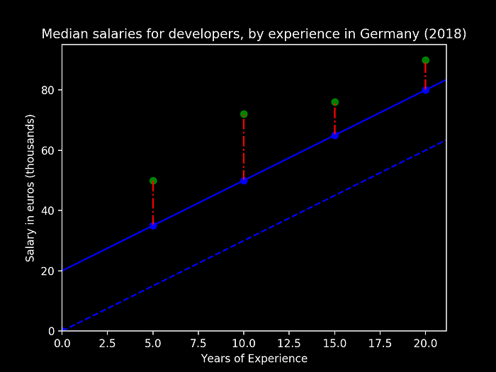
Let us consider a simple example by sampling some values from the “Developers Salaries in 2018” article from StackOverflow. Below we can see a small figure representing the average salary points, and how they evolve in Germany, as the developer experience advances in years:

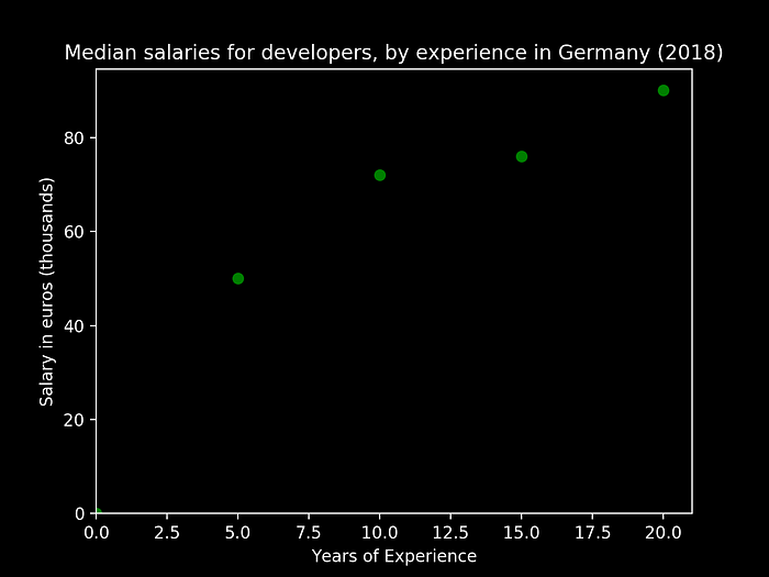
Based on the above data points, we would like to develop a simple model function that would allow us to predict how the salaries evolve at any given point of experience time.

Linear regression

A linear function can then be defined by the simple expression:

With the constant m representing the slope of the function line and b usually referred as the intercept. Some examples can be seen below for showcasing different values of (m, b):

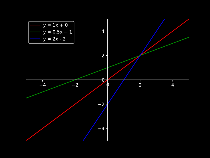
In this example above we can see that changing m influences the slope of the resultant value, as well as the intercept b who modifies the function value when crossing x = 0.

On our current scenario, as the variation of the salaries are not indeed represented by a linear progression, nevertheless, looking to the data shape on Figure 1, it would be acceptable to approximate the predicted resulting salaries by fitting a line within the points progression in a way that:

Finally, our model would try to represent itself as the line that would approximate the evolution of our parameters, salary and experience, by somehow tweaking m and b, such as it would allow us to obtain something like:

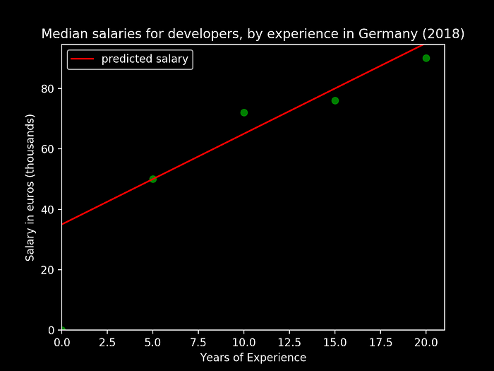
To this “linear” representation of a basic model that represents relationship between our parameters we can refer to as Linear Regression.

The Cost of our Errors

Now that we’ve identified what shape we’ll be using to generate our model we must then try to figure out what are the values of (m, b) that would better describe the evolution of our data prediction model.

But how can we choose the values of m and b that would generate us the line we search for? An approach would be to compute the errors between the values our model generates and the actual data we have in place.

A simplistic approach for representation purposes only could be:

• we know that developer with a around 10 years of experience earns around 72K euros of yearly salary (1)
• starting with a example slope and intercept of (m, b) = (3, 35)

A sample error function, for this specific data point of 10 years of experience (x=10) our error E would be:

For all of our existing sample data points, we can then compute the error that takes into account the sum of all errors between our prediction and the real value, resulting in a function as such:

with:

• n being the total samples of our data set
• y being the actual salary value for a specific observation
• x being the number of experience years that we want to predict for y

To this sum of the squared differences between each observation and its group’s mean, that would represent our Error Function (or Cost Function), we name the sum of the squared differences between each observation and its group’s mean: Sum of Squared Errors (SSE). In statistics, this mean squared error is very useful to assess the “quality” of our prediction values against real observations.

But how can we then proceed on finding the proper values for m and b? An intuitive approach could be, as we are now able to compute an Error Function, to find the pair of (m, b) that minimizes this function. If so, we can then clearly state that we have a prediction that produces the minimal error and therefore more closely represent reality.

Let us then choose two random values for (m, b), compute the cost function and then change these values to try to find the minimum of our error function. Let us consider initially (m, b) = (3, 0), and our data points from Figure 1, we obtain the following graphical result:

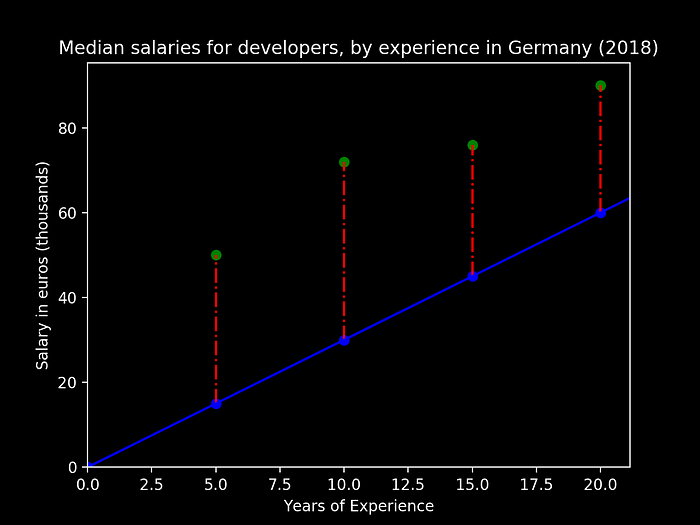
From the above figure we can see:

• the green dots representing our observed data values for the salaries
• the blue line we have our prediction model (y = 3 * years of experience + 0)
• the dotted red line represent our Error for the current parameters (m, b)

For this specific set of intercept and slope, let us now compute our accumulated cost, for the existing observations:

Let us now fix the slope value to 3 but increase our intercept to 20, (m, b) = (3, 20). We’ll obtain the following representation:

With an associated cost of E = 232.5. We can clearly see that by updating our intercept, we have improved our prediction as the error as dropped dramatically. Let us now plot multiple scenarios for different values of the intercept:

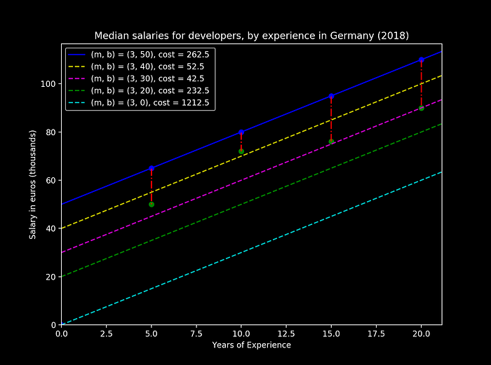
As we can see from the figure above, as we increase the value of the intercept b we can also observe the changes on the cost function. On this specific example it is trivial to identify the pink line with (m, b) = (3, 30) to be the more accurate prediction of our observed values, as it also has the lower cost value.

By plotting the variation of the error cost-function, obtained by varying the intercept value, we are presented with the following figure:

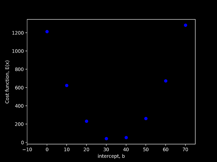
We can clearly see that, when varying the value of b, taking into account that our Error Function is convex, we are then able to find a local minimum that will represent the minimal error of our prediction model. In this simple demonstration above it is clear to state that the intercept b that minimizes our error is somewhere between [30, 40]. Unfortunately, simply iterating, with a pre-defined step, in order to find this minimum is very expensive and time consuming.

But how can we then compute this minimum of our cost function more cleverly? We’ll then be using the Gradient Descent algorithm.

Gradient Descent

The gradient descent is an iterative optimization algorithm that allows us to find the local minimums of a specific function.

A very nice example to explain the logic behind this algorithm, and recurrent in literature, is the one of the blind alpinist. Let us imagine that a blind alpinist wants to climb to the exact top of the mountain, with the least number of steps possible:

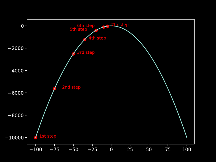
As the alpinist is blind, he will be assessing about the inclination of his current position in order to choose the magnitude of the next step he should take:

• if the inclination of the mountain (slope) of his current position is high, he can safely take a big step (as we can notice for example on the transition from the 1st step to the 2nd)
• when the slope is getting smaller, as he reaches the top of the mountain, he knows he needs to take smaller steps in order to reach approximately to the exact higher point (as the alpinist is getting closer to the top, from the 6th to the 7th step he is more careful on how to increase his position)
• for positive slopes he needs to keep on going upwards to the top
• for negative slopes, he is going down, so he needs to go back to the top

The slope of the “mountain” at a given point, is then given by the derivative of that function on a specific point:

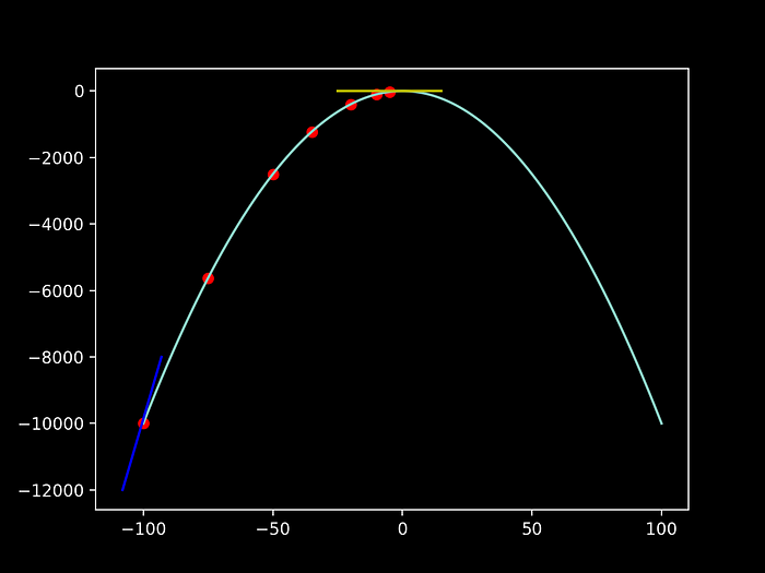
Therefore, by computing the derivative of our “mountain-function” at a certain point we can then infer about the nature of the step that we’ll be needing in order to properly reach our local minimum. By reaching a slope close to 0 (the yellow slope on the top, while compared to the blue slope value on the beginning of the mountain).

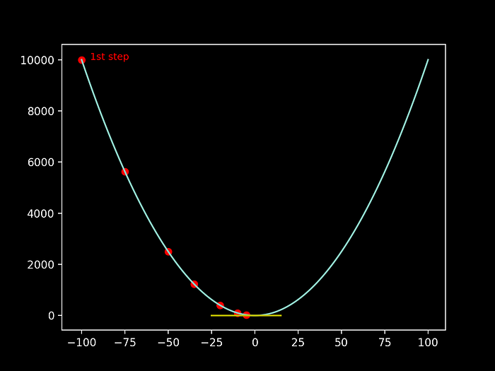
It is also trivial to understand that the same is valid for the convex version of this function, by switching the alpinist challenge from reaching the top of a mountain to actually reach the bottom of a valley:

Going back to our case of study, and taking into account that we want to to properly estimate the values of the slope and the intercept that minimize the Cost, we can then use this concept to minimize the convex function that is in fact our Cost Function.

For simplicity, let us initially just try to predict the actual value of the intercept by still keeping our slope fixed at m = 3. Our cost function would then be:

As we now know the equation of this curve, we can take its derivative and determine the slope of it at any value of the intercept.

Let us now compute the derivative of our cost function, in terms of our intercept by using the chain rule:

Now that we have properly computed the derivative we may now use the gradient descent to find where our Cost Function has its local minimum.

It would be indeed trivial to compute this specific minimum by finding the place where the derivative (slope) would be dE(b)/db = 0. Nevertheless this is not possible in many computational problems. Therefore we will apply the Gradient Descent to, starting from an initial guess, learn about the nature of this minimum. This versatility when we are unable to compute the derivative is in fact what makes this optimization algorithm so useful in so many contexts, such as modern machine learning problems.

Learning the proper value

Now that we have our derivative function, let us first compute the slope for a random value if the intercept b, such as:

With this we know that, when the intercept is 0, the slope of the tangential line on this point, on our cost function is then -69. As soon as we approach the minimum of the function, this slope would then be also close to 0.

From our alpine example we understood that the size of the step we should take should be somehow related with the slope at a given point. This has the objective of giving “bigger” steps when the slope is higher and we are far from the minimum, and giving “smaller” steps when we are getting closer to a null slope.

As we are doing this process iteratively, just us adopt the image we describe above with the actual required step sizes and adjust them on each iteration. To the constant that we will use to actually adapt the step size we call the learning rate. With this idea in mind we can defined then the following expression to generate and adapt our step size, on every iteration:

Let us assume a learning rate of 0.2, we would then obtain the following Step Size:

Taking into account our new step size, we can safely compute the next iteration intercept as being the actual step size:

So for our first iteration we have:

For this new intercept value we can see that our slope, for the error function, is then given by:

As the slope is closer to 0 we can then understand that we are actually moving closer to the optimal value just by doing a first iteration. By revisiting figure 6 we can indeed infer that by increasing the intercept from 0 to a bigger value we are indeed reducing the residual error between our estimates and the actual observations.

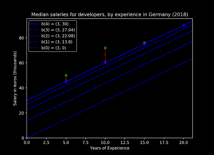
Doing a couple of iterations we obtain:

Step Size(2) = -41.4 * 0.2 = -8.28
b(2) = 13.8 - (-8.28) = 22.08
dE(22.08)/db = -24.8Step Size(3) = -24.8 * 0.2 = -4.96
b(3) = 22.08 - (-4.96) = 27.04
dE(27.04)/db = -14.8Step Size(4) = -14.8 * 0.2 = -2.96
b(4)/db = 27.04 - (-2.96)= 30
dE(30)/db = -9

We can verify from this 3 iterations the following:

• every step we are approaching a smaller absolute slope
• as we approach a 0 slope we are doing smaller steps, by keeping the same learning rate

And visually we can see that for each iteration we are getting closer to a prediction line of our data-set, and the steps are actually getting smaller:

In order to properly stop the iterations, to a certain acceptable value one should:

• decide what would be the minimal step size per iteration, e.g., stop if the step size is smaller than 0.001
• stop when we reach a certain number of iterations

By applying these rules we can verify that the algorithm stops a few iterations later:

[+] Iteration 5:Step Size = -0.592
b = 30.592
dE/db = -7.8160000000000025[+] Iteration 6:Step Size = -0.1184
b = 30.7104
dE/db = -7.579200000000007(...)[+] Iteration 9:Step Size = -0.0009472000000000001
b = 30.7397632
dE/db = -7.5204736000000025

Stabilizing with an intercept of b = 30.7397632. When plotted we obtain:

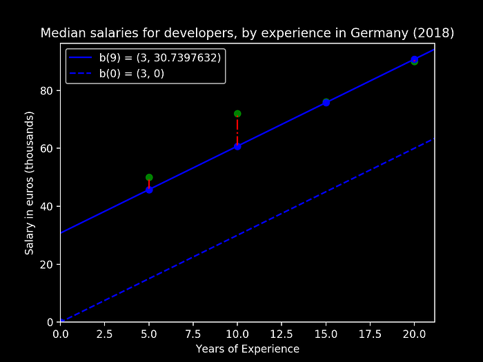
With this approach we could verify that, by iterating progressively (at the pace of adapting the step size based on a learning cave), we could indeed approach towards the minimization of the error cost function, obtaining as plotted, a very more close model representation of the evolution. This was done by simply trying to predict one of the parameters, the intercept. On the following section we will then try to understand the evolution of this model with both our variables.

Moving into the new dimension

Now that we have learned how to estimate the intercept value for our model, let us now move a step outside our one dimension and apply the gradient descent to both the intercept and the slope.

First, as on the previous section, we will then compute the derivative of our cost function, in terms of our intercept, by using the chain rule:

Now we can proceed on finding the partial derivative of our Error function in terms of the slope:

To the set of partial derivatives, to all the dimensions of this function we call then the Gradient:

We will then use this gradient, such as on the previous section to then find the local minimum of our error function. This is the reason behind calling this algorithm Gradient Descent.

In order to do it so, we need then to extrapolate what we had done for the intersect on the previous section to actually predict both values, and adjusting their own inter-dependency. Exposing it as such:

• As we are now approaching two variables, the problem could be again comparable to climbing a mountain, but with an extra dimension of complexity. You would need to adapt the pace for both the feet movement on the wall, but also a distinct one that would dictate the pace on the hands grip movement. Therefore, keeping the samelearning rate, we would then need to adapt two step sizes, one for the slope and anotherfor the intersect:

• With the new step sizes we could then obtain the current prediction for both variables, per iteration n:

• We would then compute again the gradient (namely the derivative for both variables, with the updated values):

• Repeat the whole process until we reach a choosen limit for the iterative process. We will keep on using a limit on the step size.

In order to implement this small algorithm we will need also to tweak all the initial values. A proper limit to stop value should also be decided. Let us, for our example decide on:

• the initial intersect as b = 30
• the initial slope as m = 3
• our learning rate will then be 0.001
• and we will stop when the learning rate reaches 0.00001

This can be represented by this simplistic python script:

Running this simple script we obtain the following output:

Obtaining then the following predicted values, for both our variables:

• Slope (m)= 2.5101
• Intersect (b) = 40.5478

Applying these values to our prior plots containing the error spread we obtain the following:

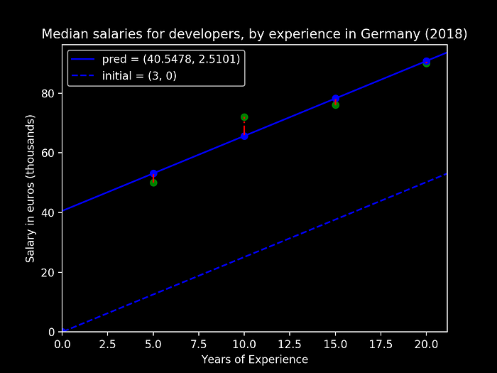
We can then see from the figure above that our (linear) prediction is now way more close to predicting the modeled data, and we could then use our new model to actually infer about the relation between these two parameters.

Conclusion

We can try to make an initial prevision about the natural relation of a set of parameters, and even obtain a simplistic model of evolution, by using Linear Regression. On this article we tried to then use this simple numerical method as a way to clearly expose the basic functioning of the Gradient Descent algorithm and mainly how we can achieve an iterative optimization of a prediction by trying to minimize a convergent error function.

Even though its owned concepts may present themselves as very simplistic, both conceptually and mathematically, they serve as one of the foundational basis to deep learning and neural networks.