Predicting AirBnB prices in Lisbon: Trees and Random Forests

In this small article, we will quickly bootstrap a prediction model for the nightly prices of an AirBnB in Lisbon. This guide hopes to serve as a simplistic and practical introduction to machine learning data analysis, by using real data and developing a real model.
It assumes as well a basic understanding of Python and the machine learning library scikit-learn, and it was written on a Jupyter notebook running Python 3.6 and sklearn 0.21. The dataset, as well as the notebook, can be obtained on my Github account, or via Google’s dataset search.
1. Data exploration and cleanup
As the first step, we start by loading our dataset. After downloading the file it is trivial to open and parse it with Pandas and provide a quick list of what we could expect from it:
Index(['room_id', 'survey_id', 'host_id', 'room_type', 'country', 'city', 'borough', 'neighborhood', 'reviews', 'overall_satisfaction', 'accommodates', 'bedrooms', 'bathrooms', 'price', 'minstay', 'name', 'last_modified', 'latitude', 'longitude', 'location'], dtype='object')
Even though above we can confirm that the dataset was properly loaded and parsed, a quick analysis of the statistical description of the data may provide us with a quick insight of its nature:
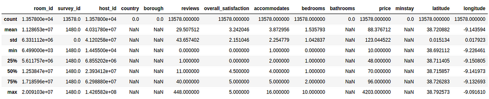
From this table, we can actually infer about basic statistical observations for each of our parameters. As our model intends to predict the price, based on whatever set of inputs we’ll provide to it, we could check for example that:
- the mean value of the nightly price is around 88 EUR
- the prices range from a minimum of 10 EUR to 4203 EUR
- the standard deviation for the prices is around 123 EUR (!)
The price distribution could be represented as follows:
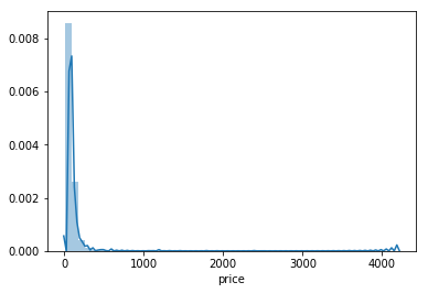
As we can see, our distribution of prices concentrates, under the 300 EUR interval, having some entries for the 4000 EUR values. Plotting it for where most of the prices reside:
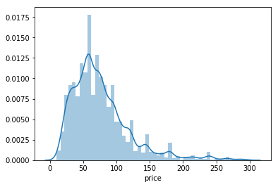
We can clearly see from our representation above that most of the prices, for a night in Lisbon, will cost between 0–150 EUR.
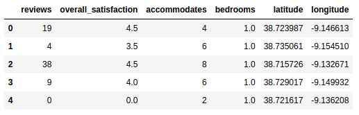
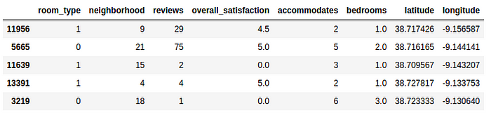
Let us now pry and have a sneak peak into the actual dataset, in order to understand the kind of parameters we’ll be working on:
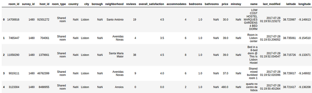
From the description above, we should be able to infer some statistical data about the nature of the data. Besides the distribution set of parameters (that we will not be looking for now), we clearly identify two sets of relevant insights:
- there are empty columns:
country,borough,bathrooms,minstay - entries like
host_id,survey_id,room_id,name,city,last_modifiedandsurvey_idmay not be so relevant for our price predictor - there are some categorical data that we will not be able to initially add to the regression of the Price, such as
room_typeandneighborhood(but we'll be back to these two later on) locationmay be redundant for now, when we have bothlatitudeandlongitudeand we may need to further infer about the nature of the format of this field
Let us then proceed on separating the dataset in:
- one vector Y that will contain all the real prices of the dataset
- on matrix X that contains all the features that we consider relevant for our model
This can be achieved by the following snippet:
With our new subset, we can now try to understand what is the correlation of these parameters in terms of the overall satisfaction, for the most common price range:
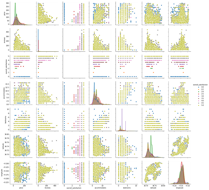
The above plots allow us to check the distribution of all the single variables and try to infer the relationships between them. We’ve taken the freedom to apply a color hue based on the review values for each of our chosen parameters. Some easy reading examples of the above figure, from relationships that may denote a positive correlation:
- the number of reviews is more common for rooms with few accommodations. This could mean that most of the guests that review are renting smaller rooms.
- most of the reviews are made for the cheaper priced rooms
- taking into account the visual dominance of the yellow hue, most of the reviews are actually rated with 5. Either this means that most of the accommodations are actually very satisfactory or, most probably, the large number of people that actually review, do it to give a 5 as the rating.
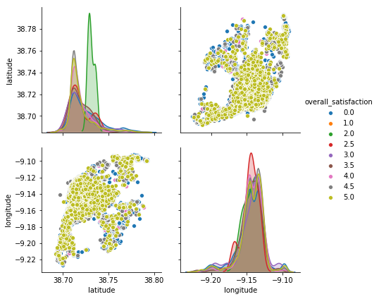
One curious observation is also that the location heavily influences price and rating. When plotting both longitude and latitude we can obtain a quasi geographical/spacial distribution for the ratings along Lisbon:
We can then add this data to an actual map of Lisbon, to check the distribution:
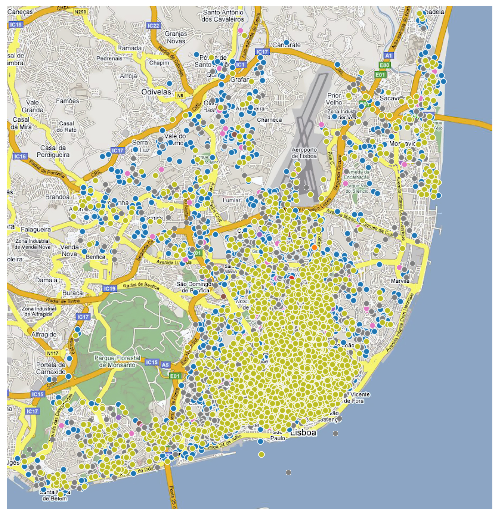
As expected, most of the reviews are on the city center with a cluster of reviews already relevant alongside the recent Parque das Nações. The northern more sub-urban area, even though it has some scattered places, the reviews are not as high and common as on the center.
2. Splitting the dataset
With our dataset now properly cleared we will then first proceed into splitting it into two pieces:
- a set that will be responsible for training our model, therefore called the training set
- a validation set that will be used to then validate our model
Both sets would then basically be a subset of X and Y, containing a subset of the rental spaces and their corresponding prices. We would then, after training our model, to use the validation set as a input to then infer how good is our model on generalizing into data sets other than the ones used to train. When a model is performing very well on the training set, but does not generalize well to other data, we say that the model is overfitted to the dataset.
For deeper information on overfitting, please refer to https://en.wikipedia.org/wiki/Overfitting
In order to avoid this overfitting of our model to the test data we will then use a tool from sklearn called https://scikit-learn.org/stable/modules/generated/sklearn.model_selection.train_test_split.html that basically will split our data into a random train of train and test subsets:
Training set: Xt:(10183, 6) Yt:(10183,)
Validation set: Xv:(3395, 6) Yv:(3395,)
-
Full dataset: X:(13578, 6) Y:(13578,)
Now that we have our datasets in place, we can now proceed on creating a simple regression model that will try to predict, based on our chosen parameters, the nightly cost of an AirBnb in Lisbon.
3. Planting the Decision Trees
As one of the most simplistic supervised ML models, a decision tree is usually used to predict an outcome by learning and inferring decision rules from all the features data available. By ingesting our data parameters the trees can learn a series of educated “questions” in order to partition our data in a way that we can use the resulting data structure to either classify categorical data or simply create a regression model for numerical values (as it is our case with the prices).
A visualization example, taken from Wikipedia, could be the decision tree around the prediction for the survival of passengers in the Titanic:
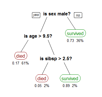
Based on the data, the tree is built on the root and will be (recursively) partitioned by splitting each node into two child ones. These resulting nodes will be split, based on decisions that are inferred about the statistical data we are providing to the model, until we reach a point where the data split results in the biggest information gain, meaning we can properly classify all the samples based on the classes we are iteratively creating. The end vertices we call “leaves”.
On the Wikipedia example above it is trivial to follow how the decision process follows and, as the probability of survival is the estimated parameter here, we can easily obtain the probability of a “male, with more than 9.5 years old” survives when “he has no siblings”.
(For a deeper understanding of how decision trees are built for regression, I would recommend the video by StatQuest, named Decision Trees).
Let us then create our Decision Tree regression by utilizing the sklearn implementation:
DecisionTreeRegressor(criterion='mse', max_depth=None, max_features=None, max_leaf_nodes=None, min_impurity_decrease=0.0, min_impurity_split=None, min_samples_leaf=1, min_samples_split=2, min_weight_fraction_leaf=0.0, presort=False, random_state=42, splitter='best')
We can verify how the tree was built, for illustration purposes, on the picture below:
Please find here a graphical representation of the generated tree @ Github.
We can also show a snippet of the predictions, and corresponding parameters for a sample of the training data set. So for the following accommodations:
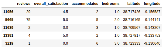
We obtain the following prices:
array([ 30., 81., 60., 30., 121.])
After fitting our model to the train data, we can now run a prediction for the validation set and assess the current absolute error of our model to assess on how well it generalizes when not run against the data it was tested.
For this, we’ll use the Mean Absolute Error (MAE) metric. We can consider this metric as the average error magnitude in a predictions set. It can be represented as such:
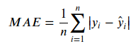
It is basically an average over the differences between our model predictions (y) and actual observations ( y-hat), making the consideration that all individual differences have equal weight.
Let us then apply this metric to our model, using Scikit Learn implementation:
42.91664212076583
This result basically means that our model is giving an absolute error of about 42.935 EUR per accommodation when exposed to the test data, out of a 88.38 EUR mean value that we collected during the initial data exploration.
Either due to our dataset being small or to our model being naive, this result is not satisfactory.
Even though this may seem worrying at this point, it is always advised to create a model that generates results as soon as possible and then start iterating on its optimization. Therefore, let us now proceed on attempting to improve our model’s predictions a bit more.
Currently, we are indeed suffering for overfitting on the test data. If we imagine the decision tree that is being built, as we are not specifying a limit for the decisions to split, we will consequently generate a decision tree that goes way deep until the test features, not generalizing well on any test set.
As sklearn’s DecisionTreeRegressor allows us to specify a maximum number of leaf nodes as a hyperparameter, let us quickly try to assess if there is a value that decreases our MAE:
(Size: 5, MAE: 42.6016036138866)
(Size: 10, MAE: 40.951013502542885)
(Size: 20, MAE: 40.00407688450048)
(Size: 30, MAE: 39.6249335490541)
(Size: 50, MAE: 39.038730827750555)
(Size: 100, MAE: 37.72578309289501)
(Size: 250, MAE: 36.82474862034445)
(Size: 500, MAE: 37.58889602439078) 250
Let us then try to generate our model, but including the computed max tree size, and check then its prediction with the new limit:
36.82474862034445
So by simply tuning up our maximum number of leaf nodes hyper-parameter we could then obtain a significant increase of our model’s predictions. We have now improved on average ( 42.935 - 36.825) **~ 6.11 EUR** on our model's errors.
4. Categorical Data
As mentioned above, even though we are being able to proceed on optimizing our very simplistic model, we still dropped two possible relevant fields that may (or may not) contribute to a better generalization and parameterization of our model: room_type and neighborhood.
These non-numerical data fields are usually referred to as Categorical Data, and most frequently we can approach them in three ways:
1) Drop
Sometimes the easiest way to deal with categorical data is… to remove it from the dataset. We did this to set up our project quickly, but one must go case by case in order to infer about the nature of such fields and if they make sense to be dropped.
This was the scenario we analysed until now, with a MAE of: 36.82474862034445
2) Label Encoding
So for label encoding, we assume that each value is assigned to a unique integer. We can also make this transformation taking into account any kind of order/magnitude that may be relevant for data (e.g., ratings, views, …). Let us check a simple example using the sklearn preprocessor:
array([3, 3, 1, 0, 2])
It is trivial to assess then the transformation that the LabelEncoder is doing, by assigning the array index of the fitted data:
array(['double room', 'shared room', 'single room', 'suite'], dtype='<U11')
Let us then apply to our categorical data this preprocessing technique, and let us verify how this affects our model predictions. So our new data set would be:
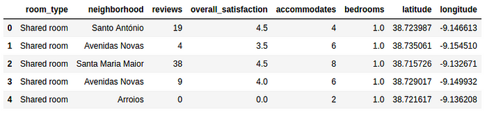
Our categorical data, represented on our panda’s dataframe as an object, can then be extracted by:
['room_type', 'neighborhood']
Now that we have the columns, let us then transform them on both the training and validation sets:
Let us now train and fit the model with the transformed data:
35.690195084932355
We have then improved our predictor, by encoding our categorical data, reducing our MAE to ~ 35.69 EUR.
3) One-Hot Encoding
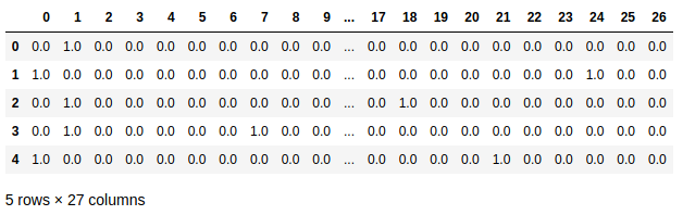
One-Hot encoding, instead of enumerating a fields’ possible values, create new columns indicating the presence or absence of the encoded values. Let us showcase this with a small example:
array([[0., 0., 0., 1., 0., 0., 1.], [0., 1., 0., 0., 0., 1., 0.]])
From the result above we can see that the binary encoding is providing 1 on the features that each feature array actually has enabled, and 0 when not present. Let us then try to use this preprocessing on our model:
So the above result may look weird at first but, for the 26 possible categories, we now have a binary codification checking for its presence. We will now:
- add back the original row indexes that were lost during the transformation
- drop the original categorical columns from the original sets
train_Xandvalidation_X - replace the dropped columns by our new dataframe with all 26 possible categories
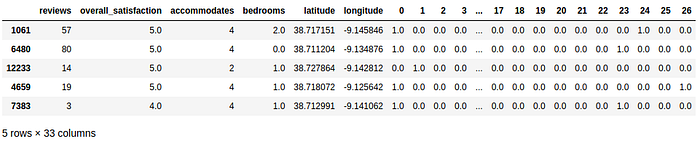
Now we can proceed on using our new encoded sets into our model:
36.97010930367817
By using One Hot Encoding on our categorical data we obtain a MAE to ~ 36.97EUR.
This result may prove that One-Hot-Encoding is not the best fit for both our categorical parameters when compared with the Label Encoding and for both parameters at the same time. Nevertheless, this result still allowed us to include the categorical parameters with a reduction of the initial MAE.
5. Random Forests
From the previous section we could see that, with our Decision Tree, we are always balancing between:
- a deep tree with many leaves, in our case with few AirBnB places on each of them, being then too overfitted to our testing set (they present what we call high variance)
- a shallow tree with few leaves that is unable to distinguish between the various features of an item
We can imagine a “Random Forest” as an ensemble of Decision Trees that, in order to try to reduce the variance mentioned above, generates Trees in a way that will allow the algorithm to select the remaining trees in a way that the error is reduced. Some examples of how the random forest is created could be:
- generating trees with different subsets of data. For example, from our set of parameters analysed above, trees would be generated having only a random set of them (e.g., a Decision Tree with only “reviews” and “bedrooms”, another with all parameters except “latitude”
- generating other trees by training on different samples of data (different sizes, different splits between the data set into training and validation, …)
In order to reduce the variance, the added randomness makes the generated individual trees’ errors less likely to be related. The prediction is then taken from the average of all predictions, by combining the different decision trees predictions, has the interesting effect of even canceling some of those errors out, reducing then the variance of the whole prediction.
The original publication, explaining this algorithm in more depth, can be found on the bibliography section at the end of this article.
Let us then implement our predictor using a Random Forest:
33.9996500736377
We can see that we have a significant reduction on our MAE when using a Random Forest.
6. Summary
Even though decision trees are a very simplistic (maybe the most simple) regression techniques in machine learning that we can use in our models, we expected to demostrate a sample process of analysing a dataset in order to generate predictions. It was clear to demonstrate that with small optimization steps (like cleaning up the data, encoding categorical data) and abstracting a single tree to a random forest we could significantly reduce the mean absolute error from our model predictions.
We hope that this example becomes usefull as a hands-on experience with machine learning and please don’t exitate to contact me if I could clarify or correct some of what was demonstrated above. There would also be the plan on proceeding on further optimizing our predictions on this specific dataset in some future articles, using other approaches and tools so keep tuned :)
7. Further reading
Please find below some resources that are very usefull on understanding some of the exposed concepts:
- StatQuest, Decision Trees: https://statquest.org/2018/01/22/statquest-decision-trees/
- Bias–variance tradeoff: https://en.wikipedia.org/wiki/Bias%E2%80%93variance_tradeoff
- Breiman, Random Forests, Machine Learning, 45(1), 5–32, 2001: https://www.stat.berkeley.edu/users/breiman/randomforest2001.pdf